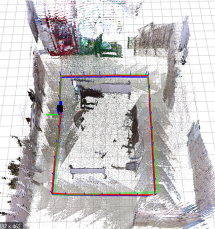
Motion planning is the soul of autonomous robot motion/navigation but given the huge variations in operational conditions, robot architecture and tasks, motion planning for robots becomes one of the most sophisticated domains of robotics.
Given the complexity of a common robot operational indoor/outdoor scene, the ideal expectation of a motion planning algorithm functional across all possible scenarios is extremely challenging. While there is enough effort put into exploiting the robot’s physical model and degrees of freedom during motion planning; there is substantial effort put into modeling the environment and its constraints as well.
For instance, navigation of a mobile robot (assumed to be a point object located at the robot’s geometrical center ) in a warehouse involves having a padding (generally equal to the robot footprint) around all the edges of the warehouse and around the obstacles because it is practically impossible for the robot’s center to go further out. Similarly, an industrial manipulator arm with fencing all around cannot obtain a pose where, though the end-effector lies within the allowed workspace has an IK configuration with a portion of the robot extruding out of the fencing.
Such intricacies necissate the formulation of different motion planning algorithms with varying assumptions and performance specifications. This article discusses the sampling-based motion planning techniques and its variants, the most used techniques implemented on mobile robots used in the industry and academia alike.
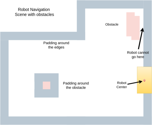
Mobile Robot Navigation Scene with Padding
Introduction
MP algorithms are generally designed knowing the limitations and demands of the environment. Also, a lot of motion planning attempts to reduce the environment and obtain a simplified version of the same for computational interpretation. Discrete search techniques are used to derive finite motion waypoints that connect the start and end. A grid-based representation of the environment is one such example, which, although promises optimality and quick solution, it is neither an adequate representation of the environment nor suitable for high dimensional state-space.
Instead of systematic discretization of the C-space and employing search algorithms, sampling-based algorithms randomly extract samples from the C-space and then construct a path out of it. Sampling-based algorithms are more useful in high-dimensional scenarios and find more optimal solutions.
Motion planning eventually is a PSPACE-hard problem where the complexity grows exponentially with C-space dimensions and gets extremely challenging with completeness and optimality requirements.
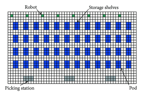
Warehouse Map - Grid Representation of the Environment
Discrete Motion Planning
It is important to acknowledge the discrete motion planning pipeline and its nuances. Despite the already mentioned limitations, discrete MP is still employed on several ocassions for ease of use and in limited complexity applications.
Discrete-search creates a discrete, finite, systematic and specific quantizated representation of the environment, obtain action-space and their involved costs and eventually employ the concerned search algorithm to find the path. They generally employ techniques like Breadth-First search, Depth-First search, A* and its variants and Dijkstra algorithms to find paths for the robot.
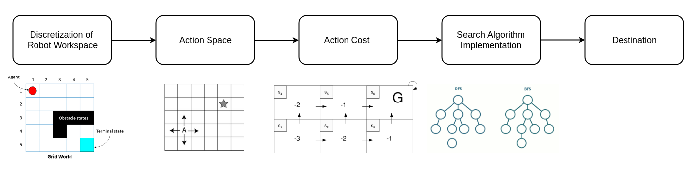
Discrete Motion Planning Pipeline
Depth-First & Breadth-First Search
Owing to the exploding nature of runtime and computational expense of search algorithms for large discrete spaces, dimensionality issues and accrual of potential inaccuracies due to the resolution of the discrete spaces; discrete motion planning becomes a non-ideal, very limited in scope technique.
Sampling-based Motion Planning
Sampling in motion planning uses the complete continuous C-space, draws samples out of it, checks the viability of the sample and eventually tries to use it to create a path towards the goal. Several assumptions and hand-crafted constraints/relaxations on performance and results help in designing very efficient real-time paths for robots.
Sampling is not affected by dimensionality of the C-space and with relaxed completeness (probabilistic completeness, i.e. asymptotic convergence) and sub-optimality conditions, it promises to be the most effective in almost all use-cases.
The Monte-Carlo methods engendered the belief in using a subset instead of all the possibilities in any state-space for search problems. Sampling-based algorithms promise better runtime performance and thus trump other more exhaustive techniques.
- Advantages - Probabilistically Complete, Applicable to High Dimensional State Space
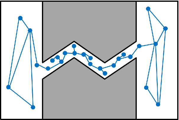
- Disadvantages - Unlike to sample narrow passages, Sub-optimal solutions
The most common sampling-based algorithms discussed here are Probabilistic Roadmaps and Randomly-Exploring Random Trees. There have been several variations proposed and used for these algorithms that have improved performance, completeness, speed and accuracy.
Sampling-based Motion Planning
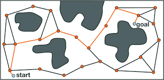
PROBABILISTIC ROADMAPS- PRM
Probabilistic Roadmap planning is a construct and multi-query motion planning technique proposed first in 1996. It has two steps - a learning phase (generally preprocessed ) and a query phase. The learning phase does the bulk work of understanding the workspace upfront before the second query phase which merely searches through the representation derived in the prior phase to provide a final solution.
LEARNING PHASE
In the learning phase - several samples are drawn from the workspace and connected to ones nearby, thus creating a roadmap between them all, including the start and desired end point. It lays the foundation for connectivity in the in the Cfree. The learning phase has a construction phase and an expansion phase.
The construction phase creates the roadmap and the expansion phase attempts at filling the gaps in connectivity between sections of the workspace positioned uniquely, involving additional sampling and connections thereafter between the disconnected components.
Learning Phase - Part I - Construction
-
Initialize the graph G(V,E) where V is the collection of nodes (the sampled points, also called milestones) and E is the collection of edges connecting certain nodes
-
Randomly sample definite number of configurations, ensure they are collision free samples and add them to V
Extracting random samples still is still tricky. Ideally, the samples should be distributed across the complete Cspace. Usually, uniform probability distribution over the particular dimension is used to ensure a map with good connectivity.
- Attempt connecting each node in V to certain, k number of other nodes and find a path between them using a local planner. The local planner can either be a fast one that tries connecting directly between the samples or a slow non-deterministic one.
If the connection is established between two nodes (the path being collision-free), the edge E(node1, node2) is saved. Generally, connectivity between the nodes is inversely proportional to the distance between them.
Missing Connections during the Construction Phase
Learning Phase - Part II - Expansion
-
Certain nodes are selected for expansion, i.e. more connectivity is attempted from those nodes.
-
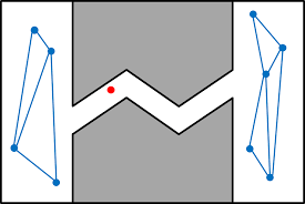
Each node n in V is assigned a weight w(n). It is an estimate of proximity of the node to difficult regions like the narrow passage shown above.
Weights are normalized such that Σw(n) = 1 and the ones with highest weights(like the red point in Figure 6) are selected to expand. If a node has poor connectivity, it should have a higher weight w(n).
- Estimation of weights for the node n can use different standards. It could be counting a certain number of nodes from V lying within a known distance radius of the node n or checking distances between a node n and its nearest connected nodes.
For the former, lower the number of connected nodes, higher the chances of the node being deserted and has poor connectivity; while for the latter, the larger distance between the node and its connected nodes, the higher connectivity gap or disconnection exists in that region.
The results from local planner connection attempts for a particular node can also be used to understand the connectivity of the same. High failure cases can be intuitively be understood as the node connected poorly or being completely disconnected. Such nodes are awarded higher weights and more connection is attempted around these.
- For the local planner,
Failure Ratio, fr(n) = f(n) / t(n) + 1
where f is the number of failures during attempted t number of connections. Finally, for one node, the weight
w(n) = fr(n) / Σ fr(a)
where fr(a) is for every node a in V
-
Finally, after the normalized weights are obtained, nodes with weights over a certain threshold are selected are expansions
- For a selected node n, at a pre-defined distance from it and in a random direction; a new node nnew is generated.
- If nnew lies in Cfree and the edge e connecting them also does, then nnew is added to V and the edge e(n, nnew) is saved in E.
- If not, the same attempt for a new node nnew is attempted in another random direction.
- At the end of expansion phase, more connectivity and ideally in inaccessible areas of the map, is obtained.
Enhanced Connectivity in Expansion Phase
QUERY PHASE
The Query Phase is a relatively easier phase with all the bulk computational processing already done. It accepts a start s and a goal g configuration and attempts to find a path between them.
Ideally, a path exists in the roadmap connecting the two and the query returns that path (a collection of all intermediate edges passing through other intermittent nodes that eventually establish connectivity between s and g)
-
If the start s and goal g are points not already sampled and existing in the roadmap R, they are connected to the closest nodes in R, through paths Ps and Pg. If these two connections are not possible, the complete query fails for path the between s and g does not exist.
-
Starting with s, new nodes with increasing distance from it are added to the path P being derived, using a local planner again.
-
Finally, the complete path connecting is given as Pcomplete = Ps + P + Pg
Given that there are several parameters, assumptions and challenges like number of samples, number of retries, sampling techniques, local planners, narrow passages in the map and sampling near obstacles; there are chances of the query failing.
However, limited connectivity in the roadmap and all problems are attempted to be resolved by retrying Learning Phase, exhaustively running Expansion Phase and concurrently operational Learning & Query Phases.
There are several enhanced PRM techniques like Obstacle-Based PRM, Medial-Axis PRM and Simplified PRM among others used to address specific challenges for sampling near obstacles, sampling in narrow passages and sampling problems in general.
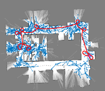
RAPIDLY-EXPLORING RANDOM TREES
Rapidly-Exploring Random Trees (RRT) is the most famous family of sampling-based motion planning algorithms. While PRMs or Potential Field methods are probabilistic in nature and have limitations with substantial effect on planning, RRTs can solve better for lots of constraints.
The algorithm basically starts at some location in the map and starts branching out in random directions, sampling new points at pre-defined distance from the initial location. After an edge is established between the initial point and the new sampled point, the latter becomes the initial location for the next step of branching out.
Using appropriate values for step size, number of sampels to drawn, initial point and other parameters, a densely connected tree-structured map is promised.
The Algorithm
-
Setup the planner with an initial point xinit, the number of points to be sampled k and the step size Δt
-
Initialze a tree τ that shall contain sampled points, with the initial point xinit
-
Sample a random point xrand in the workspace
-
Obtain the nearest neighbor xnear for the xrand point from the list of points in τ
-
Finally, derive a new point xnew and add it to the tree τ If distance (xnear , xrand) is less than step size Δ, then xnew = xnear, else xnew is an intermittent point at a distance of Δ from xnear on the line joining xnear and xrand.
-
The edge e(xnear, xnew) is an intermittent path in the tree. Several short paths like these ensure connectivity throughout the map
-
If the distance(xnew, xgoal) is less than the step size Δ, the edge e(xnear, xnew) is also stored as a path.
-
Final points in τ are all possible nodes in the map.
Salient Features of RRTs
*RRTs can solve for holonomic, nonholonomic and kinodynamic situations. Kinodynamic planning is when the robot planning is done within the kinematic constraints of velocity, acceleration, joint angle limits and obstacle avoidance.
-
In cases where a naive random tree is generated out of incrementally selecting random points and adding it to the vertices, it heavily explores an already clustered environment.
-
Even a random walk shows bias towards already explored places. Since, RRT is generated by selection of the nearest vertex, it ensures unexplored sections of the configuratio space are considerably seen.
-
RRTs do not form closed loops and thus, the map it decides is near optimal if not completely optimal.
-
Initially, the vertices are not uniformly distributed but the probability of a random point lying withing the step size deltat of a vertex of a tree(the xnear point) eventually tends to 1
-
If the random points generated are uniform, then such a setting would be independent of xinit and would defy the purpose of RRTs.
-
Also, if the points are sampled from some pre-defined PDF (probability distribution function), then the RRT vertices would be accordingly. Such a setup can be used to device biased schemes which might be difficult and time taking to converge.
-
Ideal performance of a RRT is defined by the distance parameter Δ - which determines the shortest distance between two states.
-
For constrained path planning, the optimal path would be the one with the least cost function and the cost function would be its metric.
-
Probabilistic approach creates too many extra edges and also depends upon k-nearest neighbors as compared to a single neihbor for the RRTs.
-
RRT is probabilistically complete and relatively easier to implement.
-
RRT maps always remain connected even in cases of less vertices and can be applied to a broad range of planning algorithms.
Given the advantages of the basic RRT algorithm, several enhancements like Bidirectional RRT, RRT, RRT-Connect and RRT-Smart among others have been used to optimize the solutions and get better performance.
Recently, lots of efforts have been put into using RRT with better hardware (like GPUs), using other search algorithms in conjunction and hand-crafted optimizations for certain operational constraints/desires have fetched roboticists enhanced performance and usage.
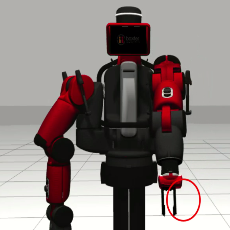 Baxter Kinematics & Dynamics Library