Simultaneous Localization & Mapping is the domain of robotics that forms the pillar for autonomous navigation in mobile robots of all kinds and even self-driving cars. As the name suggests, SLAM involves mapping (creating computationally viable representation of the environment) and localization(determination of robot’s pose in the environment), at the same time. It is like a chicken-and-the-egg problem - a map is needed to localize the robot pose on it and the pose is needed to estimate the map. It is the most applicable in GPS denied environments or environments where a task needs to be done at higher accuracy than the GPS provided map information.
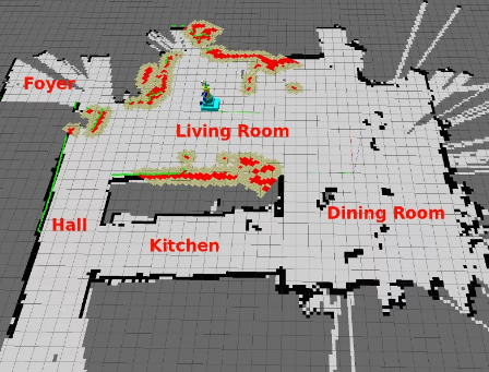
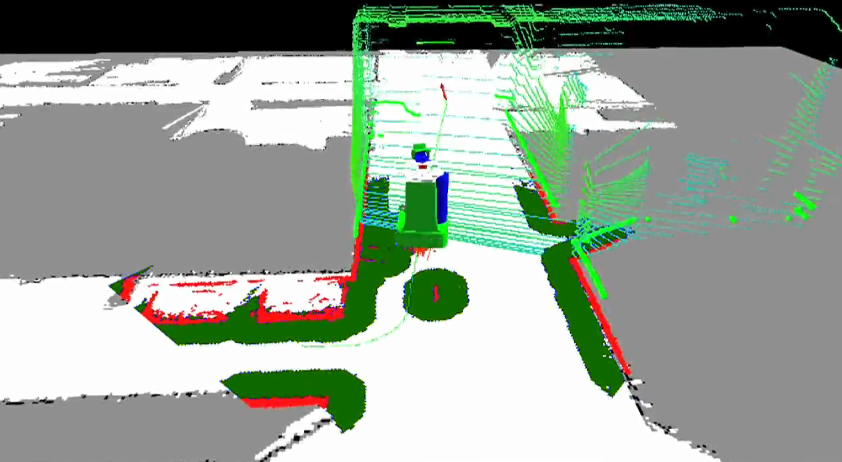 Sample of a SLAM operational PR2 robot
Introduction
SLAM is used for locomotion tasks in indoor as well as outdoor applications. Moroever, there are applications of the same in robotic manipulation and humanoids. The robot pose is the robot’s position (x, y, z) coordinates with reference to the origin and the orientation of robot’s heading. Mapping is modeling of the environment in different ways. Estimating one among the pose or the map when the other is given is easy but simultaneous estimations with uncertain priori is extremely difficult. So, the results obtained are highly stochastic and thus the entire process is aimed at making decisions that enhance the probabilities.
Using observed landmarks, estimates of maps and sensor-based information; the complete navigation SLAM is implemented. The sensor-based information includes deriving landmarks in the scene (like edges of the wall as seen by a camera) or other features of the map like the possible relative positioning of landmarks or otherwise.
SLAM as expected is a highly stochastic setup and probabilistic techniques are largely used. The stochasticity in solutions is reduced by using closed-loop solutions, i.e. relating the landmarks and features by comparing it against the ones that the robot has already visited. Meticulous perception systems are needed to establish relationships between unknown map elements, features and landmarks.
Mapping
Maps are representations of a scene and can be done in several ways for robot to interpret. For instance, a human-readable definition of a map for a desert would be sand all around, then an oasis in the center and then a few bushes around; a robot needs to know a lot more and the nuances and in a computationally defined format. These maps are generally 2D and can be easily extensible to 3D format. There are two main categories of maps - metric maps and topological maps. Metric maps are analogous to political maps of a city while topological maps are the physical maps of the same place.
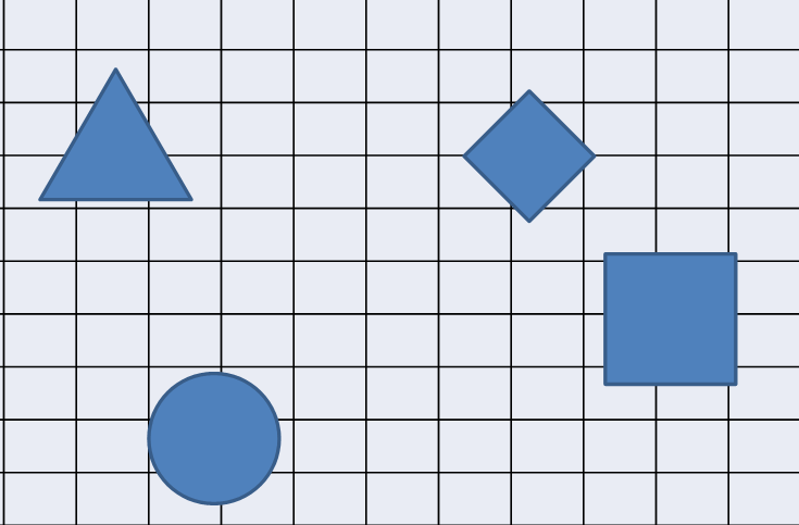 Sample Robot Map - Occupany Grid Map
- Metric Maps
Metric maps are geometric representations of the surroundings with known edge sizes and area scaled as per real world. Occupany grids are the most common form of metric maps where the complete area is decomposed into several smaller units with information about if the map is occupied by anything or free for robot motion. While the ease of creating occupancy grids makes them preferrable for general applications, large storage and processing power is needed to process all individual grids at every iteration. Dynamic variation of grid sizes(collapsing several smaller grids into one large grid) is useful in overcoming these limitations. Grids maps are useful for motion and path planning algorithms like A* or Djisktra as they have low computational costs. Occupancy probability definition for each sub-grid in the large grid makes the map diffcult to obtain for practical use with large areas.
- Topological Maps
Topological maps are description of the robot environment in terms of physical features. For an indoor environment, it would be landmarks and features like rooms, electrical appliances and furniture. The path to locations are proposed as sections in the map that can be accessed by the robot. The features are called nodes while the connecting paths are called edges or connections. These maps require verbose knowledge of the environment and are generally used in visual SLAM.
Localization Algorithms
Localization is a map dependent definition of robot’s pose that determines. For a known map, known sensor observations and location estimates, robot localization is very much possible. The quality of localization with higher probabilities for correctness highly depends on sensor readings. Thus, more the sensors, better the localization sensing.
A robot can bes easily localized using information from exteroceptive and interoceptive sensors like range finders and IMUs respectively, processed over time.
- Localization Algorithms
Robot localization is generally solved using algorithms like Kalman Filter, Extended Kalman Filter and Particle Filters. KF and EKF solve for linear and non-linear systems respectively, by using the system model and the related covariances. Extended Kalman Filtering is generally the most used algorithm that supports multiple sensor data usage and provides accurate robot pose.
Particle filter is a setup where each unique particle represents a probable robot pose with some associated probability of being the robot’s actual pose. Thereafter, the SLAM algorithm can use the mean, average or highest probability value as the robot pose. Large number of particles results in more computational overhead.
- Robot Pose Types
A robot’s pose is generally defined in a frame of reference, i.e. the origin of a map. Onboard sensors are good for measuring the robot’s own motion and thus the relative pose estimation of the robot with reference to the previous can be obtained. Wheel encoders are used for odometry estimation. They measure the rotations in each motor and use the robot’s model to obtain the motion information (change in position and change in orientation). The other way is using inertial measurement units that use accelerometers, gyroscopes andd magnetometers and integrate the measurements to estimate the motion. However, each of these sensing options have their own limitations. Wheel encoder based odometry are prone to huge errors due to slipping, uneven ground and drifting as well as inherent sensor inefficiencies. IMUs are prone to drift and bias accumulation over time. The estimations are made based on integrations and thus prone drift
Given the volatality of maps and thus everything derived from it, absolute pose estimation of a robot in a map is extremely difficult and inextensible as the map is still in evolution. The unknown nature of surroundings makes it difficult to localize on the absolute level. Absolute positioning is done by laser rangefinders or GPS, both of which are very limited in scope and usage. While it is not prone to any accumulating errors, the absolute estimations can be marred by sensor issues and limited sensors.
Nuances of SLAM
SLAM techniques run with only certain physical parameters. It includes u - the robot control input, z - the sensor observations, m - the environment map and x - the robot pose or path.
Feature-based SLAM methods analyze the surroundings, create the maps, obtain close-to-accurate robot poses and thus converge onto motion tasks. It needs absolute robot poses, absolute positions of the landmarks but only relative measurement of the landmarks.
Measurements and estimations in SLAM are cyclic. So, an error in robot pose leads to an imperfect estimate of the map that eventually results in a poor robot pose calculated thereafter; eventually, showing that they are correlated. Also, the mappings between the observations and the actual landmarks are unknown.
SLAM could be operational as full SLAM, online SLAM and integral SLAM. Full SLAM estimates the complete path(sequence of poses) and the full environment map while online SLAM estimates pose for the latest time stamp using the old information and the complete map. Integral SLAM does recursive computations, one at a time. Thus, full SLAM computes sets of u, z, x and final m while online SLAM computes u_last, z_last, and the complete map m.
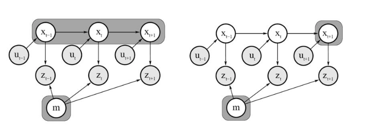 Full SLAM vs Online SLAM
Sensors in SLAM
Interoceptive and exteroceptive are two broad categories of sensors comprising of onboard sensors like wheel encoders, IMUs and GPS and cameras and laser scanners respectively. Interoceptive sensors are supposed to measure the physical quantities of the robot itself while the exteroceptive sensors observe the outer world and each of them thus contribute towards robot’s pose estimation. Sonars, lasers and cameras are the three most used exteroceptive sensing systems used in SLAM.
Sonars and lasers use time of flight and phase-shift based computations to determine the contents and the structure of the environment, the map. LiDARs rangefinders have long ranges and high operational speeds to determine planar features like walls in the environment. 2D LiDARs can only determine planar features while 3D LiDARs can determine the complete environment due to the highly dense information available. However, LiDARs cannot observe surface properties to localize and identify objects. Thus, LiDARs are more emphatically used to determine locations of obstacles and bounds of the environment.
Visual sensing using monocular cameras, stereocameras and RGB-D cameras suffice to compensate for the limitations of the LiDARs. While cameras can provide rich information, processing the same is computationally expensive and needs more time and more complex algorithms to obtain computer legible data. Visual Odometry estimation and visual landmark estimation are the most useful SLAM applications for camera information. Monocular vision lacks depth information for the contents in the image thus making 3D map reconstruction very difficult. While there have been attempts are obtaining depth information based on robot motion and consecutive frames of images, it is still limited by complex algorithms and real-time computations. The depth information even obtained after this is associated with an unknown or probably incorrect scaling factor that mars the direct use in motion.
Stereovision is today’s easiest option to obtain the depth information for the surroundings. It uses the triangulation method on two monocular cameras of known focal lengths, setup at a known distance and that determines the depth of any pixel in real-world physical quantities.
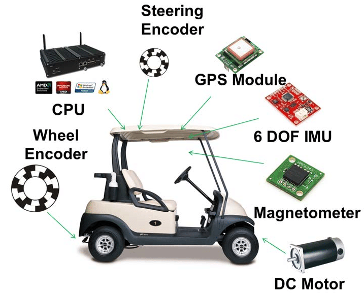 Different Sensors on a mobile robot
Sensor Fusion
Both pose estimation techniques are mutually exclusive but several sensor-fusion techniques are used to compensate for the limitations in the individual sensors. Sensor fusion can be performed at sensor level as well as at the approach level. Multiple sensor data feed can be either fused together before estimating the pose or individual estimations can be fused later on.
The position measure can be fused using a probabilistic framework like Markov Localization or Kalman Localization. Markov Localization predicts(using the several sensors and their relative and/or absolute measurements) the pose information as a probability over all possible locations while Kalman localization predicts the same as a probability over the complete map thus making the location with highest chances have the largest probability.
Given the pose of a robot is 6DOF (x, y, z position coordinates and alpha, beta and gamma orientation coordinates), it becomes really difficult to estimate each of them accurately and their corelation makes accuracy challenging.
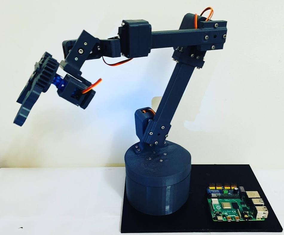 FumbleArm - 6DoF Manipulator Arm