Bayesian methods discussed earlier were a preface to the use of different probabilistic techniques in robotics. Bayesian inference derives the final equation that presents the various steps involved in the process of state-estimation by using the action and the model of the system.
The Kalman filters family is used for linear as well as non-linear models with Gaussian noise distribution assumption. This family of filters is most widely used for non-critical tasks where several assumptions and relaxed approximations can be used during noise or system modeling. While Kalman filter works well for linear models, the Extended Kalman filter is capable of working on non-linear models by the potential use of linearization of the models.
This article is a walkthrough of the application of the Extended Kalman Filter for robot localization. The content is primarily derived from the excellent tutorial SLAM for Dummies by Søren Riisgaard and Morten Rufus Blas.
Introduction
The Extended Kalman Filter is the go-to algorithm for state estimation for non-linear models with well-defined transition models. It works on non-linear state transition and observation models while assuming the process and observation noise both to be multivariate Gaussians.
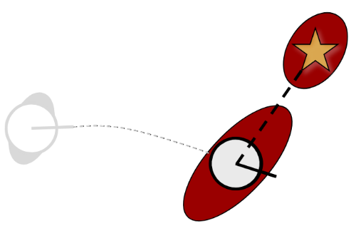
Robot localization is the process of finding the robot’s pose(position and orientation) with respect to a given map. Given the stochasticity in robot motion, sensors, and environment interaction, localization is a very sophisticated task. EKF is largely deployed in SLAM algorithms to use the odometry information and the landmarks in the environment for localization. The landmarks are represented as point objects with position (xl, yl) as the cartesian position coordinates.
Representation of the different components of localization
The EKF technique uses feature extraction, landmarks generation, data association, odometry, and landmark representation and sensor data concepts. Here is a glance at them individually after which, the setup should be ready to implement EKF.
-
Sensor Data: The laser scanner or LiDAR is used here to obtain information about the world. The laser scan gives the range (distance between the target and the sensor) and the bearing (alignment of the corresponding line of sight for the measurement). It is usually represented as [range, bearing] and the bearing value is basically a multiple of the angular resolution of the scanner.
-
Odometry: Odometry data uses the robot’s initial pose, motion information from the wheel encoders(over a finite time span) and the robot kinematic model to predict the robot’s new pose. It may also use the control input or the data from an onboard IMU sensor for the same.
-
Landmarks: Landmarks are those distinct features in the environment that can be used to get a sense of the robot’s pose in the environment. These are essentially re-observable features like the edge of the walls or furniture in the environment, patterns on the walls and more. Landmarks should essentially be re-observable from different locations in the environment, distinguishable from each other, ideally stationary and enough in quantity to create a stable map covering the complete environment.
- Landmark Extraction: Given that we are using the laser scan data to extract the landmarks in the environment, it is important to define what features we are looking for and expecting. Laser scans give the range and the bearing information over the field of view which is used in primarily two ways to determine landmarks.
-
If the difference in range values for two consecutive or very closely positioned readings is larger than a threshold, it suggests the presence of a small/point obstruction, which is called a spike landmark. While it is easy to compute, it is prone to errors due to sensor anomalies and not feasible for surroundings with smooth curvature.
- Random Sampling Consensus (RANSAC) is a more sophisticated technique used to determine patterns and curvature of the surroundings. For RANSAC, the sensor readings are converted from polar coordinates (range, bearing) to cartesian coordinates (x, y) and then; S points are randomly sampled from these and the least-squares approximation is used to fit a line on these S points. Thereafter, the proximity of the points to this line is obtained and if there is a high consensus(above a set threshold) of points close to this line, it is probably a landmark( maybe a wall), and a better fit is found for all these consensus points.
This best fit line is a landmark and the point on this line closest on the robot, is an equivalent point landmark.
- Data Association: After landmarks have been extracted from the sensor readings, the most crucial step is to identify if the current landmark has already been observed or is a new one. It is crucial to associate the landmark correctly to avoid erratic beliefs in robot’s pose. A new landmark is compared against all existing landmarks in the database using the neared-neighbor technique and if their proximity is within the error ellipse, they are essentially the same landmark that has been reobserved.
Main components of EKF localization
EKF localization has three significant steps; state estimate prediction, state estimate update, and addition of landmarks. While there are several intermediate steps, these three steps are the highlight of the complete state estimation cycle.
- Prediction: Estimate the current state using the information from the odometry and/or the IMU. It is considering the input to the robot and the model-based expected/observed motion to predict the robot’s current state.
New pose: (x,y) –>(dx, dy) (x + dx, y + dy)
- Update: Use the information from the landmarks to update the state estimate. This involves several intermediate steps.
When the sensors observe the world, feature extraction techniques are employed to determine if there are landmarks in the surrounding. Using data association techniques, observed landmarks are compared to existing landmarks. If a match is found, the difference in positions of the landmarks (position prediction based on the robot’s pose prediction against position observed by the sensing system) acts as the innovation component. The innovation is used to update the robot pose estimate.
For re-observed landmarks, this step also updates the belief in those landmarks and updates their uncertainty matrices defined later.
- Landmark Addition: Based on observations in the previous step, if the landmark observed does not match any old landmark and is completely new, it is added to the database of existing landmarks.
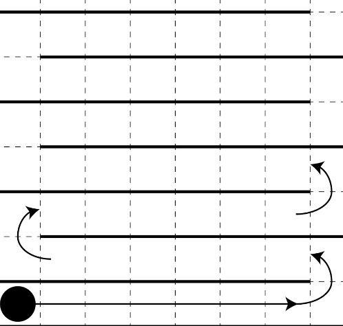
 Mobile Robot Kinematics