Control techniques in robotics can largely be classified as model-based and model-free. The most common control techniques include PID, gain-scheduling, cruise-control, adaptive control, robust control and reinforcemment learning-based control among others. Majority of the model-based control techniques have an upper-hand over the model-free techniques as the former estimate control signals with some information about the response expected from the plant.
The model-free techniques like PID or other ML and AI based techniques, need a lot of training to develop the same extent of fidelity as model-based techniques. However, model-based techniques are prone to modeling errors while system identification and modeling in itself is a very strenous process and model-free techniques do not have such requirements. Model-free techniques deriving the tuning parameters during the training procedure are essentially deriving a pseudo-plant model in the backend that helps them know the correct relationshop between the input and output.
 Examples of Control Techniques
Introduction
Model predictive control is an advanced control technique that manipulates the plant output while also satisfying the set of constraints and handling disturbances. MPC is an online technique which is essentially an optimization problem for the objective function defined for the desired plant output. MPC uses the plant model and predicts the control signals for a finite set of future timestamps corresponding to the desired output. However, it only implements/executes inputs only for a small fraction of the predicted timestamps and repeats the process at the next prediction timestamp.
MPC can handle the dynamics of the highly non-linear systems and the unanticipated disturbances as well. It can operate on MIMO (multi-input multi-output) systems with constraints on the system properties. As MPC can look into the future predictions, it can also handle unexpected disturbances. However, it is a computationally expensive method and with increasing system complexity, the compute power requirement can increase exponentially.
It is often known as receding horizon control or dynamical matrix controlor generalized predictive control.
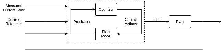 MPC Flowchart
Common Applications Of MPC
MPC is straightforward genralized control technique that can handle a lot of constraints, variations, disturbances and almost all system given the model, thus making it suitable control technique for a lot of applications from industry and products to academia and more.
Common applications of MPC include:
- Trajectory Control for vehicles
- Process Control for manufacturing factories
- Missile guidance systems
- Space navigation
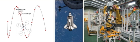
MPC Applications
Functional Aspects Of MPC
MPC uses the model of the system and solves an optimization problem attempting to find the global minima for the defined objective function also called cost function. The optimization task is an interative process that finds the most favorable set of input signals that minimize the error in desired and predicted output while also satisyfing the set of constraints. The sequence of control inputs steer the system towards the desired setpoint response. At each timestep, the controller solves an open-loop optimization problem and after it applies the first control signal generated, the output is fedback as system state for optimization for the next timestep.
An MPC may not necessarily be optimal as the optimization solvers are prone to local-minimas but it ensures that the system converges to the best possible and feasible solution.
MPC has a few design parameters which need to be either selected carefully or learned by experience to obtain the best performance of the controller.
-
Sample Time - Ts It is the time period at which the controller executes the control algorithm and sends the instructions to the system. Larger sample time means the system’s ability to respond to unknown disturbances is poor and smaller sample time means the controller is very computationally heavy. Thus, the optimal value of the sample time should be the system rise time, i.e. the time in which the system response rises from 10% to 90% of the desired steady-state output. If the sample time is very low, lower than the mechanical response time of the system; the system doesn’t have enough time to act on the current input signal and the new signal arrives thereby creating undesired behavior.
-
Constraints on variables There could several physical limits on the different inputs and outputs as well as their rate of change, in the system that the optimization should take into consideration. Such constraints are useful in maintaining smooth response, non-impulsive and infeasible behavior of the system.
-
Weights for different components of the objective function Because there are several constraints and goals to be achieved, it is difficult to quantitatively present the goal priority in the optimization task. In an MPC, weights are defined for ratio between different output goals, or between the outputs and the inputs or between different soft constraints that could be bent a little.
-
Prediction Horizon It is the number of the timesteps over which the optimization should be done while predicting the control inputs. The larger the prediction horizon, the more computationally expensive does the system get while the lower the predicted horizon, the poor the optimization efficiency and ability to look into the future. It is the number of timesteps the controller looks into the future and usually 20-30 time samples, each of timestep Ts.
-
Control Horizon It is a certain number of timesteps into the future that the optimizer derives as the moves that have significant impact on the system’s attempt to converge to the desired output. It is usually chosen as 10-20% of the predicted horizon.
Sample MPC Problem
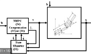
A typical multivariate control system using an MPC controller operates on the system model, usually non-linear, a cost function and an optimization algorithm. Usually, the problem is a convex optimization task and that should be optimized for prediction horizon.
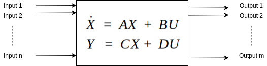
State-Space Model of Control Systems
For a given discrete time state-space model like shown above, the typical cost function could be:
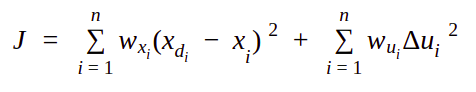
Sample Cost function for a common non-linear function
In the cost function above,
- i is the current timestamp and n is the total prediction horizon
- xdi is the desired output for the particular timestamp i while xi is the system current state
- wxi is the weight of the desired/reference output at the particular timestemp i
- wui is the weight of the rate of change of input at the particular timestemp i
- Δui is the weight of the rate of change of input at the particular timestemp i
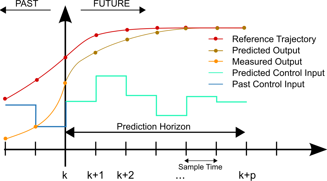 MPC Time Graph
Types of MPC
MPC is largely dependent on the model of the system and while it may be easy to model simple automation systems, it gets extremely complicated to design dynamic systems like robots and their non-linearity is difficult to solve for the MPC. There are several complexities in systems as well, which tend to disturb the dynamics and expected responses from it. To accomodate such variations or adapt to changing operational evnironment or to ease the MPC implementation, different types of MPC are deployed.
-
Linear MPC - The simplest implementation of an MPC where if the model is linea and the constraints are linear, then MPC optimization cost function could be a QP problem and be solved easily using a linear time-invariant MPC. The problem becomes a simple convex optimization task with a global minima and no more complexities.
-
Adaptive MPC - If the system model is non-linear, while the constraints and the cost function are still linear, the model can be linearized at each operating point (computationally expensive step though) and same method as above could be implemented. Because the MPC adapts to the system at each time step, this is called adaptive MPC.
-
Gain Scheduling MPC - It is more coarse version of the adaptive MPC and analogous in behavior to the gain scheduling used in PID contro. Instead of the system being linearized at each operating point, gain-scheduling MPC linearizes the function over diffeerent segments in the operational range offline and then implements a linear MPC switching between the different linearized models depending on the system state.
-
Nonlinear MPC - If the cost function, system model and the constraints are all non-linear, non-linear MPC is deployed. It is very prone to local minimas due to the non-convex optimization task and may result in sub-optimal solutions.
Model Predictive Control is a very powerful tool for controling the system response and is widely used in robotics. It finds major applications in autonomous vehicle trajectory tracking and control. It has also been researched for, in manipulation and aerial navigation. Part II of this series explains the application of MPC in robotics with an implementation for the same, in C++. Stay tuned!
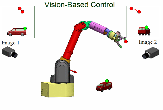 Visual Servoing For Manipulators - Part I